A cautionary tale on imputation with random forest
Missing data and imputation methods
Missing data is ubiquitous in data science and has the potential to significantly impact results if not handled properly. Historically, three primary mechanisms for missing data have been defined:
- Missing completely at random (MCAR): the probability of missingness is the same for all observations.
- Missing at random (MAR): the probability of missingness depends on observed variables.
- Missing not at random (MNAR): the probability of missingness depends on unobserved variables.
As a side note, with the rise of big data and increased interoperability, new types of missingness have emerged that do not fit into this traditional classification. One such type is structured missingness¹Mitra, R., McGough, S.F., Chakraborti, T. et al. Learning from data with structured missingness. Nat Mach Intell 5, 13–23 (2023). https://doi.org/10.1038/s42256-022-00596-z, which occurs when datasets with different sets of variables are integrated.
Several methods are available for handling missing data, each with its particular strengths and weaknesses, such as mean and median imputation, missing indicator method, regression imputation, among many others. In this study we will focus only on two methods, the gold standard multivariate imputation by chained equations (MICE)²Stef van Buuren, Karin Groothuis-Oudshoorn. mice: Multivariate Imputation by Chained Equations in R. Journal of Statistical, (2011). https://www.jstatsoft.org/article/view/v045i03 implemented in the R package "MICE", and the machine learning based method fast imputation with Random Forest "miceRanger" package.
Both methods featured here use multiple imputation, but they differ significantly in two aspects. First, MICE uses a linear regression model to impute missing values, while miceRanger uses a Random Forest (RF) model. Second, MICE uses Gibbs sampler with Markov Chain Monte Carlo (MCMC) for sampling the joint distribution, while miceRanger uses empirical cumulative distribution function (ECDF) for sampling. The latter is the more robust approach as it attempts to model the whole joint distribution of the data.
The first aspect means that because of the nature of RF, miceRanger allows the introduction of non-linearities and agnostic interactions during the imputation process. This comes with the price of a larger sample size requirement for reducing overfitting and more hyperparameters to be tuned for the imputation.
The aim of this analysis is: 1) compare the coefficient of determination \( R^2\) and 2) regression coefficient estimates \( \hat{\beta}_i\) after MICE and miceRanger imputation. We will verify if miceRanger can provide unbiased estimates for a linear regression model fitted on MCAR data and how it compares with classical MICE estimates.
Simulation
We generated three sets of 100 datasets, each containing 1000 data points, with covariates \( (x_1, x_2) \) drawn from a bivariate distribution of means \( \vec{\mu }= (1, 80) \), standard deviations \( \vec{\sigma} = (10, 30) \) and covariates correlation \( \rho = 0 \), giving the following variance-covariance matrix:
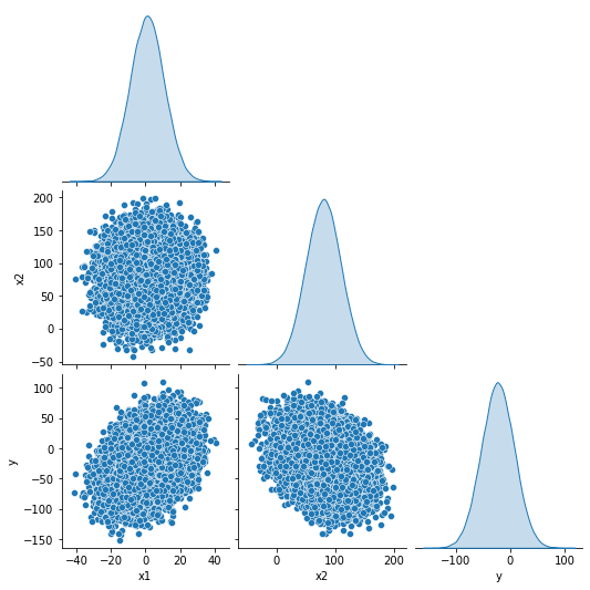
The response is given by \( y \equiv \beta_0 + \beta_1 x_1 + \beta_2 x_2 + \varepsilon \) with \( \vec{\beta} = (0, 1, -0.3) \). We control the coefficient of determination \(R^2\) by tuning the amount of gaussian noise \( \varepsilon \sim \mathcal{N}(0,\,\sigma_{\varepsilon}^{2})\) in the model. The three complete sets of data provide linear models with \(\hat{R^2} = (0.2, 0.5, 0.8) \) respectively. In summary, the data points are generated according to a linear model with specified means, standard deviations, coefficients, and \( R^2 \) value. Fig. 1 (a) depicts the response and independent variable distributions and their relationship.
We then apply amputation to introduce missing values in the simulated data using the MCAR mechanism. For each dataset we create three different versions with missing rates of \(0.2\), \(0.5\) and \(0.8\), accounting for 900 datasets in total. In Fig. 2 (b) we show the missing pattern used to generate the amputed data, only one missing variable is allowed per observation. In Table 1 we summarise the different conditions explored in this study.
 (b)
(b)

Table 1: Datasets with different missing rates and \(R^2\) values. In total we have 9 conditions with 100 replicates each. Show Table 1
Results and discussion
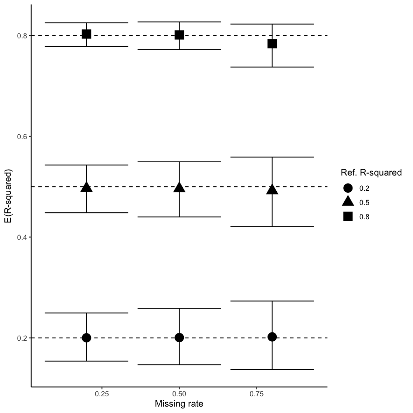
The Figure 2 shows coefficient of determinations for different correlations and missingness degree estimated with linear regression after MICE and miceRanger imputation. For MICE, we see that the confidence intervals always cover the true value of \(R^2\) and the mean estimate is close to the true value independent of the strength of the correlation between the response and covariates, and the amount of missingness in the data. The confidence intervals are bigger for higher amount of missingness due to increased uncertainty, as expected.
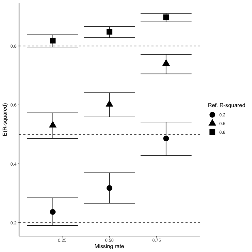
On the other hand, we can see that performances obtained with miceRanger are always overestimated, which indicates that the imputation method is introducing a stronger correlation than the true relationship in the data. This problem becomes exacerbated for high amount of missingness (50 and 75%) where the true value is not covered by the confidente interval.
To investigate this problem further we run another simulation where there is no correlation between the response variable and the covariate. We trained Random Forest and linear regression models. Fig. 3 shows the predicted points along with the original data for both methods. We see that Random Forest overfitted to the training data and predicts values close to the original data, even though there is no correlation in the original data. The \(\hat{R^2}\) are \(0.80\) and \(0.16 \times 10^{-3}\) for RF and LR, respectively.
Fig. 4 shows how estimated parameters are affected when data is imputed using MICE (left) and miceRanger (right) with data generated under intermediate correlation, R² = 0.50. For MICE, we see that the confidence interval becomes larger as the amount of missingness increases, but the true value remains covered. On the other hand, estimates from miceRanger exhibit a huge effect overestimation and small confidence intervals that do not cover the true value, indicating that the imputation method introduces a stronger correlation.

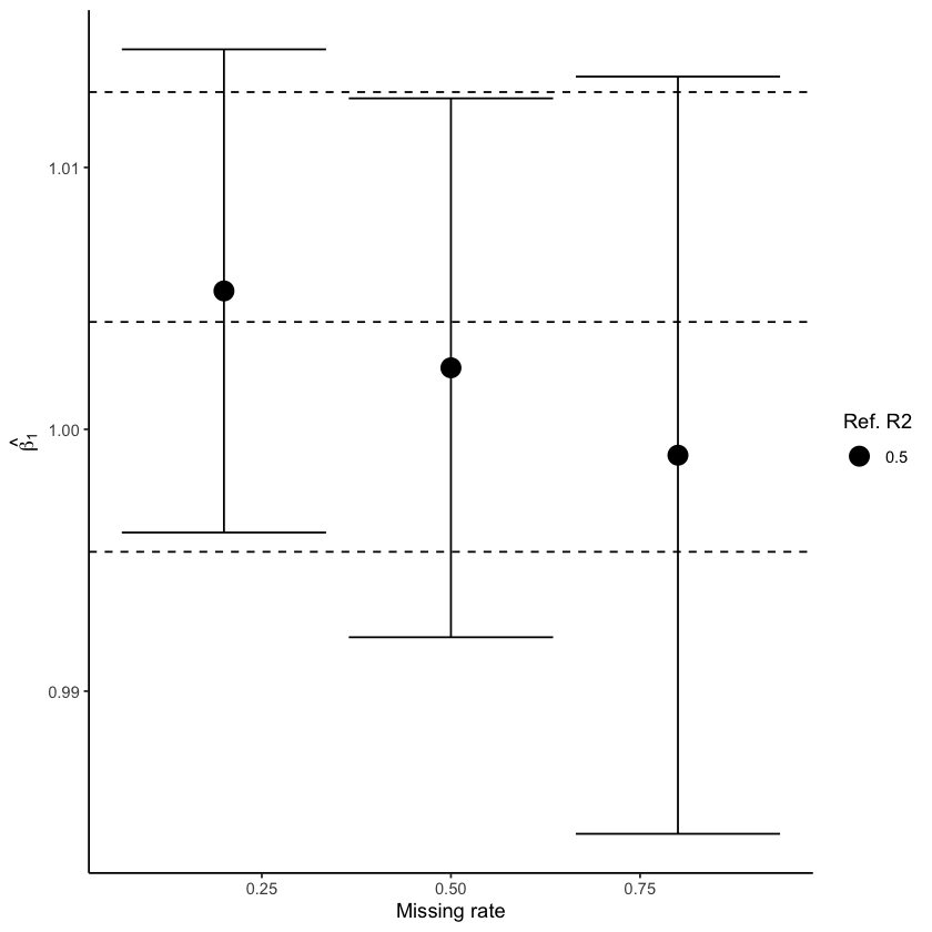
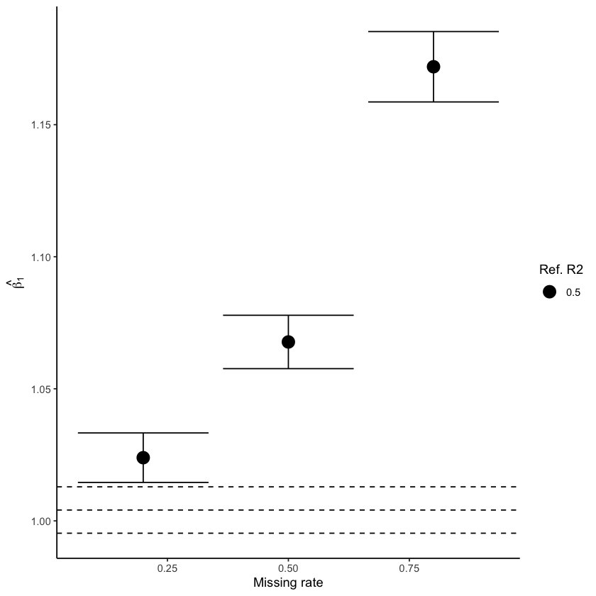
Figure 4: Estimated parameter values obtained using MICE (left) and miceRanger (right) for data with intermediate correlation \(R² = 0.50\). Dashed lines represent the true value and CI estimated without missing values.
Conclusion
We argue that RF-based methods have the potential to overfit to previously seen data which is dangerous when applied to imputation in classical inference studies. New imputation methods developed with this class of estimators require careful evaluation w.r.t their impact on parameter estimation. We observed that spurious correlations and interactions can be introduced during the imputation phase, affecting results further in the analysis pipeline with high risk of bias.
We strongly advocate for directing efforts towards developing theoretical guarantees for newly created ML-based imputation methods. It is essential that we bridge the gap between the rapid pace of tool development and the need for rigorous theoretical foundations, including statistical guarantees. By doing so, we can ensure the scientific community has confidence in the reliability and effectiveness of these innovative approaches, ultimately accelerating their adoption and impact.
References
Mitra, R., McGough, S.F., Chakraborti, T. et al. Learning from data with structured missingness. Nat Mach Intell 5, 13–23 (2023). https://doi.org/10.1038/s42256-022-00596-z
Stef van Buuren, Karin Groothuis-Oudshoorn. mice: Multivariate Imputation by Chained Equations in R. Journal of Statistical, (2011). Software. https://www.jstatsoft.org/article/view/v045i03