Internal validation with bootstrap .632+ estimator
Introduction
Internal validation is an important step in model development. The aim of internal validation is to estimate model performance on unseen data drawn from the same population where the model was developed. On the other hand, external validation is performed by an independent¹Internal-external validation is when the same group that developed the model uses independent data for model validation. group of researchers using independent data. It is important to note that internal validation often gives better performance than observed on new data, considering that population shift is a common issue.
We will briefly present different internal validation methods and focus on the bootstrap .632+ estimator. Bootstrap is a powerful statistical method not only in the context of prediction models but also in hypothesis testing, confidence interval estimation, and many other applications. The main idea behind bootstrap is that we resample from the original data to estimate the distribution of an estimate. In the context of internal validation, it allows for estimating the least biased performance of a given model compared to split-sample and cross-validation methods.
At the end of this post, we will provide a simple example using the bootstrap .632+ estimator to evaluate a logistic regression model for breast cancer prediction.
Split-sample
The most common and simplest validation method is the split-sample, which involves splitting the data into training and testing sets (see Fig. 1). When using the split-sample method, the best practice is to develop the model using only the training set, completely blind to the test set, and only use it to evaluate the model performance as the last step in the analysis. The split-sample method is popular in big data and machine learning due to the computational cost of applying other validation methods. Cross-validation and bootstrap become prohibitive for large sample sizes (\(N > 10000\) samples), in high-dimensional settings, and when complex algorithms such as neural networks are employed.
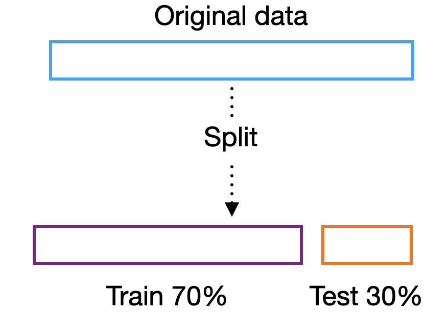
Figure 1: Split-sample scheme in train and test set. In this example, 70% of the data is reserved for model development and 30% for internal validation.
Nonetheless, the split-sample method has several pitfalls with serious consequences for model development. The first issue is that we are not using the whole data to develop our model, and in small sample size settings, it can impact model performance. If the whole data is used for re-training the model after internal validation, we end up with a model that is not the same as the one tested. The performance is sensitive to the choosen split which is prone to gaming, the split can be changed until the best performance is achieved. Several studies have delved into the weaknesses of the split-sample method, and the recommendation is that it should not be used in studies where the sample size is less than tens of thousands (Steyerberg, E. W., 2019).
\(k\)-fold Cross-validation
Cross-validation is more robust than the split-sample method. The data is divided into \(k\) folds, where \(k-1\) folds are used for training and the remaining fold is used for testing (see Fig. 2). The process is repeated \(k\) times, each time a different fold is used for testing. The final performance is the average of the \(k\) performances. The 5- and 10-fold cross-validation are the most common settings, but other values of \(k\) can be used. For instance, leave-one-out cross-validation (LOOCV) is often applied to very small data (\(N < 100\)), where \(k=N\) and only one value is used for validation at a time. Cross-validation can be computationally expensive depending on the number of folds, but it is a good compromise between the split-sample method and bootstrap.
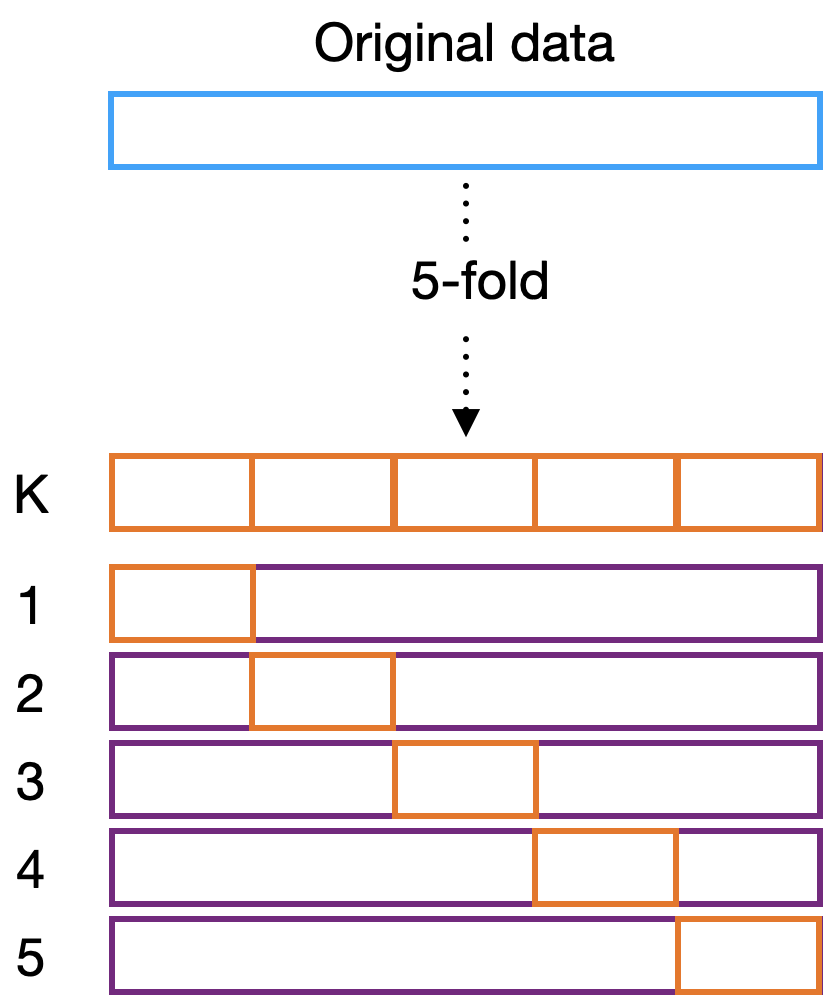
Figure 2: 5-fold cross-validation scheme. For each k-fold, we have the training set represented by the purple region and the test set in orange. In this case, models are developed in 4/5 of the data and tested in 1/5 of the data for each fold.
Bootstrap
The original data \(D_{\mathrm{orig}}\) contains \(N\) samples. Bootstrap internal validation employs resampling with replacement, which means that the \(k^{\mathrm{th}}\) resample \(D_{\mathrm{BS}}^k\) will contain the same number of samples \(N\) as the original data, but by chance, some observations will be selected more than once and some will not be selected at all. The observations not selected are part of the out-of-bag (OOB) sample \(D_{\mathrm{OOB}}^k\). Statistically, around 63.2% of the subjects are represented in each resample and 36.8% are included in the respective OOB samples. Figure 3 depicts how the data is resampled.
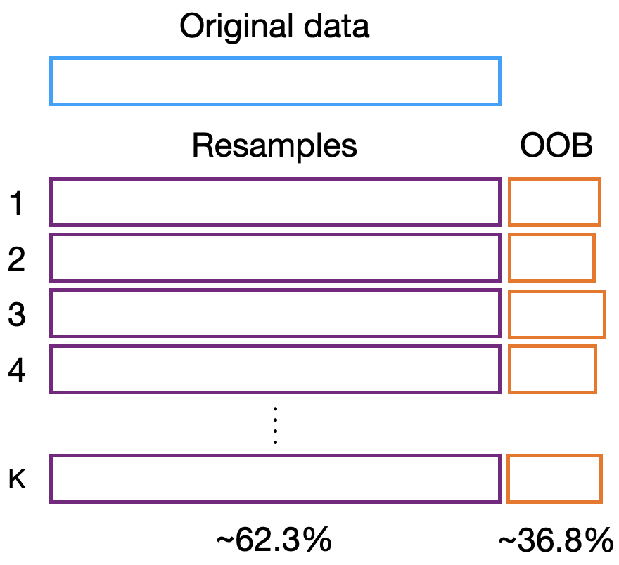
Figure 3: Bootstrap internal validation scheme. The data is resampled k-times with replacement, which means that the sample size of each bootstrap is the same as the original data. The out-of-bag (OOB) contains the cases that were not included in each resample. The resamples will contain approximately 63.2% of the data.
The main model \( \hat{\mu}_{\mathrm{orig}}\) is trained on the original data \(D_{\mathrm{orig}}\). The model is evaluated with a given metric \( \hat{\theta}\) on the same data, which will of course provide a highly optimistically biased estimate of performance \( \hat{\theta}_{\mathrm{orig}, \mathrm{orig}}\), where the first subscript identifies the data in which the model was trained and the second the data where the model was evaluated. For each resample \(k\), we train a model \( \hat{\mu}_{\mathrm{BS}}^k\) which will be evaluated on the OOB data \( \hat{\theta}_{BS, OOB}^k\). The evaluation of the models on the OOB data will produce pessimistic estimates of model performance.
Efron (1983) proposed the .632 estimator, which combines the performances obtained on the original data and in the resamples and attempts to reduce the upward bias:
$$ \theta_{.632} = 0.368 \hat{\theta}_{\mathrm{orig}, \mathrm{orig}} + 0.632 \langle \hat{\theta}_{\mathrm{BS}, \mathrm{OOB} } \rangle $$where \( \langle \theta_{\mathrm{BS}, \mathrm{OOB} } \rangle \) is the mean for all resamples.
This estimator brought a significant improvement compared with the state of the art at that time, but it was shown that it is actually downwardly biased.
To provide a less biased estimate, the .632+ estimator was proposed by Efron (1997). This new estimator incorporates different weights \( \omega \) to the .632 estimator by taking into account the performance of a non-informative model \( \gamma \) to define the relative rate of overfitting \( R \). For example, for binary classification where the metric of interest \( \theta \) is the ROC AUC, we would set our non-informative performance as \( \gamma = 0.5\). For continuous regression models, the non-informative model could be chosen as a model that always predicts the mean. Thus, the .632+ estimator is defined as:
$$ \theta_{.632+} = (1-\omega) \hat{\theta}_{\mathrm{orig}, \mathrm{orig}} + \omega \langle \hat{\theta}_{\mathrm{BS}, \mathrm{OOB} } \rangle, $$with the relative overfitting rate:
$$ R = \frac{\langle \theta_{\mathrm{BS}, \mathrm{OOB} } \rangle - \theta_{\mathrm{orig}, \mathrm{orig}}}{\gamma - \theta_{\mathrm{Orig}, \mathrm{Orig} } }, $$and weight:
$$ \omega=\frac{.632}{(1-.368R)}. $$Example: Breast cancer prediction model
We illustrate the .632+ estimator with a simple example. We will use the Breast Cancer dataset from the scikit-learn library. The dataset contains 569 samples and 30 features. We will use a logistic regression model to predict the target variable, which is binary. The performance metric of interest is the ROC AUC.
If you want to implement this example as an exercise, we recommend to structure the code in the following way:
- A function to obtain the resamples and store the indices in a dataframe
- Two functions to obtain the bootstrap data and the out-of-bag data
- Implement the bootstrap .632+ estimator
- Write a simple pipeline to train the main logistic model and a loop for all bootstrap models
- Check the mean OOB performance, the confidence intervals, and the .632+ performance estimate.